

Mixed Effects Model (Single-trait)
Contents
17. Mixed Effects Model (Single-trait)#
Consider the mixed linear model
where \(\boldsymbol{\beta}\) is a vector of fixed effects, \(\mathbf{X}\) is an observed matrix that relates \(\boldsymbol{\beta}\) to \(\mathbf{y}\), \(\mathbf{u}\) is a vector of multivariate normal random effects with null means and covariance matrix \(\mathbf{G}\sigma^2_u\), and \(\mathbf{e}\) is a vector of multivariate normal residuals with null means and covariance matrix \(\mathbf{R}\sigma^2_e\). The fixed effects are usually assigned a flat prior distribution, and the matrices \(\mathbf{G}\) and \(\mathbf{R}\) are assumed to be known. The variance components \(\sigma^2_u\) and \(\sigma^2_e\) will be assigned scaled inverted chi-square prior distributions with scale parameter \(S_{u}^{2}\) and degrees of freedom \(\nu_{u}\) for \(\sigma^2_u\) and parameters \(S_{e}^{2}\) and \(\nu_{e}\) for \(\sigma^2_e\). As described in Sorensen and Gianola (2002), the Gibbs sampler can be used to construct a Markov chain that has the posterior for the unknowns in the model as its stationary distribution. This is accomplished be sampling from the full-conditional posteriors of the unknowns. The derivations presented below closely follow those in Sorensen and Gianola (2002).
Then, the joint posterior for all the unknowns, denoted by \(\boldsymbol{\theta}\), is
17.1. Full-conditional posterior for location parameters#
We show below that the full-conditional distribution for the location parameters in the model, \(\boldsymbol{\theta}_1' = [\boldsymbol{\beta}', \mathbf{u}']\), is normal with mean given by the solution to:
and variance-covariance matrix given by the inverse of the coefficient matrix of (1).
For convenience, we will write the above equation as:
where \(\mathbf{W} = \begin{bmatrix}\mathbf{X} & \mathbf{Z}\end{bmatrix}\) and \(\mathbf{D}\) is a block diagonal matrix that adds zero to the diagonals of \(\mathbf{X}'\mathbf{R}^{-1}\mathbf{X}\) and \(\mathbf{G}^{-1}\) to \(\mathbf{Z}'\mathbf{R}^{-1}\mathbf{Z}\).
The full-conditional posterior for \(\bs{\theta}_1\) is
which can be recognized as a normal distribution with mean \(\hat{\bs{\theta}}_1\) and covariance matrix \((\mathbf{W}'\mathbf{R}^{-1}\mathbf{W} + \frac{\sigma_{e}^{2}}{\sigma_u^2}\mathbf{D})^{-1}\sigma^2_e\), assuming that \((\mathbf{W}'\mathbf{R}^{-1}\mathbf{W} + \frac{\sigma_{e}^{2}}{\sigma_u^2}\mathbf{D})\) is non-singular.
17.2. Single-site Gibbs Sampling of Fixed and Random Effects#
If we denote the location parameters (\(\boldsymbol{\beta}, \mbf{u}\)) of the model by \(\boldsymbol{\theta}\), as we have seen before, the posteior distribution of \(\boldsymbol{\theta}\) is multivariate normal with mean given by the solution to
and the variance is \(\mbf{C}^{-1}\sigma^2_e\), where \(\mbf{C}\) and \(\mbf{r}\) are the coefficient matrix and right-hand-side of the MME. So, the quadratic in the exponent of this normal distribution is:
In order to use the single-site Gibbs sampler to construct a Markov chain for \(\boldsymbol{\theta}\), we need to derive the full-conditional posterior distribution for \((\theta_i|\text{ELSE})\), where \(\text{ELSE}\) stands for all other variables in the model other than \(\theta_i\). To simplify this derivation, \(\boldsymbol{\theta}\) is partitioned as:
where \(\boldsymbol{\theta}_1 = \theta_i\) and \(\boldsymbol{\theta}_2\) contains the remaining elements of \(\boldsymbol{\theta}\). Now, the quadratic (2) can be written as:
where the coefficient matrix \(\mbf{C}\) has also been partitioned to correspond to the partitioning of \(\boldsymbol{\theta}\).
To derive the distribution of \((\boldsymbol{\theta}_1|\boldsymbol{\theta}_2)\), we need to only consider the terms in (3) that involve \(\boldsymbol{\theta}_1\). These terms are (after dropping \(\frac{-1}{2\sigma^2_e}\)):
where for (4) to equal (5), \(\tilde{\boldsymbol{\theta}}_1\) must satisfy the equality:
This equality must hold for all \(\boldsymbol{\theta}_1\), and so
because the right-hand-side of the MME corresponding to \(\hat{\boldsymbol{\theta}}_1\) is equal to
Thus, \((\boldsymbol{\theta}_1|\boldsymbol{\theta}_2) \sim \text{N}(\tilde{\boldsymbol{\theta}},\mbf{C}_{11}^{-1}\sigma^2_e)\). An alternative derivation is given in Sorensen and Gianola (2002).
17.2.1. Gibbs Sampler for Location Parameters#
function Gibbs!(A,x,b,varRes::Float64,nIter::Int64;outFreq=100)
    n = size(x,1)
    xMean = zeros(n)
    for iter = 1:nIter
        if iter%outFreq==0
            println("at sample: ",iter)
        end
        for i=1:n
            cVarInv = 1.0/A[i,i]
            cMean   = cVarInv*(b[i] - A[:,i]'x) + x[i]
            x[i]    = randn()*sqrt(cVarInv*varRes) + cMean
        end
        xMean += (x - xMean)/iter
    end
    return xMean
end
Gibbs! (generic function with 1 method)
17.3. Estimation of Variance Components#
17.3.1. Full-conditional posteriors for \(\sigma^2_u\) and \(\sigma^2_e\)#
In the joint posterior, \(\sigma^2_u\) appears only the density of \(\mbf{u}\) (p1) and in its scaled inverted chi-square prior (p2). Thus, the full-conditional posterior for \(\sigma^2_u\) is:
which can be recognized as having the form of a scaled inverted chi-square distribution with degrees of freedom \(\tilde{\nu}_u = \nu + k\) and scale parameter:
A random variable from this distribution can be obtained as: \(\frac{(\mbf{u}'\mbf{G}^{-1}\mbf{u} + \nu_uS_u^2)}{\chi^2(\tilde{\nu}_u)}\), where \(\chi^2(\tilde{\nu}_u)\) is a chi-square random variable with \(\tilde{\nu}_u\) degrees of freedom.
Similarly, it can be shown that the full-conditional distribution for \(\sigma^2_e\) is a scaled inverted chi-square with degrees of freedom \(\tilde{\nu}_e = n + \nu_e\) and scale parameter:
17.4. Coding#
17.4.1. Structures for Building MME#
using DataFrames, SparseArrays, LinearAlgebra, Random, JWAS, CSV, Printf, Statistics, Plots, Distributions, ProgressMeter

mutable struct ModelTerm
    trmString::AbstractString
    startPos::Int64
    endPos::Int64
    randomType::String
end

mutable struct RandomEffect
    modelTermVec::Array{ModelTerm,1}
    νpr::Float64
    Spr::Array{Float64,2}
    Vi::Array{Float64,2}
    meanV::Array{Float64,2}
    Ai
    estimate::Bool                # new
    outSamples::Bool              # new
    outFreq::Int64                # new
    outStream                     # new
end

mutable struct MME
    modelEquation::AbstractString           #"y = A + B + A*B"
    covVec::Array{String}                   #["age"]
    modelTermVec::Array{ModelTerm,1}        #[modelTerm("A") , modelTerm("A*B")]
    modelTermDict::Dict{AbstractString,ModelTerm}
    randomEffectsVec::Array{RandomEffect,1} #[RandomEffect("Ind"), RandomEffect("Mat")]
    ped                                     # false or a pedigee structure defined in JWAS.PedModule
    depVar::Symbol                          #:y
    X::SparseMatrixCSC{Float64,Int64}       #design matrix
    mmeLhs::SparseMatrixCSC{Float64,Int64}  #left-hand side for MME
    mmeRhs::Array{Float64,1}                #right-hand side for MME
    mmeSpl::Array{Float64,1}                #sample of location effects              # new
    varRes::Float64                         #residual variance
    νRes::Float64                           #prior degrees of freedom for varRes     # new
    SRes::Float64                           #prior scale parameter for resVar        # new
    y::Array{Float64,1}                     #vector of values for dependent variable # new
    meanVarRes::Float64
end

function ModelTerm(str::AbstractString)
    ModelTerm(str,0,0,"fixed")
end
ModelTerm
17.4.2. Functions for Building MME#
function initMME(modelEquation::AbstractString,varRes;νRes=5.0)  # "y = A + A*B"
    if modelEquation==""
        error("modelEquation is empty\n")
    end
    leftRight  = split(modelEquation,"=")       # "y", "A+A*B"
    depVar     = Symbol(strip(leftRight[1]))    # :y
    modelParts = strip(leftRight[2])            #"A+A*B"
    termsVec   = split(modelParts,"+")          #"A","A*B"
    modelTermVec = [ModelTerm(strip(trmStr)) for trmStr in termsVec]
    modelTermDict = Dict{AbstractString,ModelTerm}()
    for i in modelTermVec
        modelTermDict[i.trmString] = i
    end
    randomEffectsVec = []
    ped = false
    covVec = []
    X = spzeros(0,0)
    mmeLhs = spzeros(0,0)
    mmeRhs = []
    mmeSol = []
    y      = []
    SRes   = varRes*νRes/(νRes-2)                            # new
    meanVarRes = 0.0                                         # new
    return MME(modelEquation,covVec,modelTermVec,modelTermDict,randomEffectsVec,ped,
               depVar,X,mmeLhs,mmeRhs,mmeSol,varRes,νRes,SRes,y,meanVarRes)
end
initMME (generic function with 1 method)
# This function returns returns a dictionary with the names in the pedigree as the keys and their
# sequential numbers as the associated values
# It also returns vector with the keys in sequential order.

function mkDict(ped::JWAS.PedModule.Pedigree)
    d = Dict()
    names = Array{String}(undef,length(ped.idMap))
    for i in ped.idMap
        d[i.first] = i.second.seqID
        names[i.second.seqID] = i.first
    end
    return d,names
end

# This function returns
# a dictionary with the unique values in the vector "a" as the keys and their
# sequential numbers as the associated values
# It also returns vector with the keys in sequential order.
function mkDict(a)
    d = Dict()
    aUnique = unique(a)
    names = Array{String}(undef,size(aUnique,1))
    for (i,s) in enumerate(aUnique)
    names[i] = s
    d[s] = i
    end
    return d,names
end

function getX(mme,modelTerm::ModelTerm,covariables,df)
    n = size(df,1)
    trmString = modelTerm.trmString
    if trmString == "intercept"
        X = ones(n,1)
        colNames = ["intercept"]
        return X,colNames
    end
    factors = strip.(split(trmString,"*"))
    covs = [i in covariables for i in factors]

    if covs[1] == false
        str = string.(df[:,Symbol(factors[1])])
        val = 1.0
    else
        str = fill(factors[1],n)
        val = df[:,Symbol(factors[1])]
    end

    for i in 2:length(factors)
        if covs[i] == false
            str = str .*" x ".*string.(df[:,Symbol(factors[i])])
            val = val .* 1.0
        else
            str = str .*" x ".*fill(factors[i],n)
            val = val .* df[:,Symbol(factors[i])]
        end
    end
    dict,colNames   = modelTerm.randomType != "A" ? mkDict(str) : mkDict(mme.ped)
    str = modelTerm.randomType != "A" ? str : string.(df[:,Symbol(factors[1])])
    ii = 1:n                     # row numbers
    jj = [dict[i] for i in str]  # column numbers
    p = length(colNames)
    X  = sparse(ii,jj,val,n,p)
    return X, strip(modelTerm.trmString)*": ".*colNames
end
getX (generic function with 1 method)
function setRandom!(mme::MME,trmStrings::String,V,ped=false;
                estimate::Bool=false,                          # new
                νPrior::Float64=4.1,                           # new
                outSamples::Bool=false,                        # new
                outFreq::Int64=100                             # new
            )
    m = size(V,1)

###################### new ############################################
    if outSamples==true
        fileName = "V($trmStrings).samples"
        outStream = open(fileName,"w")
        for i=1:m,j=i:m
            if i==j==1
                @printf(outStream,"%6s", "V[$i,$j]")
            else
                @printf(outStream," %6s", "V[$i,$j]")
            end
        end
        @printf(outStream,"\n")
    else
        outStream = nothing
    end
#######################################################################

    var = m==1 ? fill(V,1,1) : V
    trmVec = strip.(split(trmStrings,[',';' '],keepempty=false))
    if length(trmVec) != size(var,1)
        println("size of var: $(size(var,1)) does not match the number of random effects: $(length(trmVec))")
        return
    end
    modelTerms = [mme.modelTermDict[trm] for trm in trmVec]
    if ped==false
        [trm.randomType = "I" for trm in modelTerms]
        Ai = I
    else
        [trm.randomType = "A" for trm in modelTerms]
        mme.ped = pedigree
        Ai = JWAS.PedModule.AInverse(pedigree)
    end
    Spr = (νPrior - m - 1)*var                                                  # new
    randomEffect = RandomEffect(modelTerms,νPrior,Spr,inv(var),zero(var),Ai,    # new
                        estimate,outSamples,outFreq,outStream)
    push!(mme.randomEffectsVec,randomEffect)
end

function addGiMats!(mme::MME)
    for randomEffect in mme.randomEffectsVec
        for (i,modelTermi) in enumerate(randomEffect.modelTermVec), (j,modelTermj) in enumerate(randomEffect.modelTermVec)
            starti = modelTermi.startPos
            startj = modelTermj.startPos
            endi = modelTermi.endPos
            endj = modelTermj.endPos
            mme.mmeLhs[starti:endi,startj:endj] = mme.mmeLhs[starti:endi,startj:endj] + randomEffect.Ai*randomEffect.Vi[i,j]*mme.varRes
        end
    end
end
addGiMats! (generic function with 1 method)
function getLhsRhs!(mme,df)
    X,colNames = getX(mme,mme.modelTermVec[1],mme.covVec,df)
    mme.modelTermVec[1].startPos = 1
    mme.modelTermVec[1].endPos  = mme.modelTermVec[1].startPos + size(X,2) - 1
    for i = 2:size(mme.modelTermVec,1)
        Xi,namesi = getX(mme,mme.modelTermVec[i],mme.covVec,df)
        X = [X Xi]
        mme.modelTermVec[i].startPos = mme.modelTermVec[i-1].endPos + 1
        mme.modelTermVec[i].endPos   = mme.modelTermVec[i].startPos + size(Xi,2) - 1
        colNames = [colNames; namesi]
    end
    y = df[:,mme.depVar]
    mme.X = X
    mme.mmeLhs = X'X
    mme.mmeRhs = X'y
    mme.mmeSpl = zero(mme.mmeRhs)
    mme.y      = y
    addGiMats!(mme)
    return mme.mmeLhs,mme.mmeRhs,colNames
end
getLhsRhs! (generic function with 1 method)
function updateLhs!(mme)
    mme.mmeLhs = mme.X'mme.X
    addGiMats!(mme)
end
updateLhs! (generic function with 1 method)
17.4.3. Numerical example#
pedigree = get_pedigree("simData.ped",separator=",",header=false);
The delimiter in simData.ped is ','.
Pedigree information:
#individuals: 1248
#sires:       50
#dams:        198
#founders:    248
data = CSV.read("data.phen",DataFrame)
first(data,5)
| Ind | Mat | y | |
|---|---|---|---|
| Int64 | Int64 | Float64 | |
| 1 | 251 | 177 | 3.896 |
| 2 | 252 | 192 | -1.739 |
| 3 | 253 | 64 | 2.729 |
| 4 | 254 | 191 | 2.894 |
| 5 | 255 | 127 | 4.331 |
varRes = var(data[:,3])/2.0
13.747279059434936
varGen = varRes
13.747279059434936
mme = initMME("y = intercept + Ind",varRes);
setRandom!(mme,"Ind",varGen,pedigree,estimate=true);
lhs,rhs,names = getLhsRhs!(mme,data);
17.4.3.1. Known variance components#
x = zero(rhs);
nIter = 50000
solGibbs = Gibbs!(lhs,x,rhs,varRes,nIter;outFreq=10000);
at sample: 10000
at sample: 20000
at sample: 30000
at sample: 40000
at sample: 50000
QRLhs = qr(lhs)
sol = QRLhs\rhs
[names solGibbs sol]
1249×3 Matrix{Any}:
 "intercept"  -1.4949     -1.47888
 "Ind: 1"     -1.85365    -1.87255
 "Ind: 38"     0.281539    0.243685
 "Ind: 125"   -0.298755   -0.320123
 "Ind: 519"    0.577422    0.552815
 "Ind: 16"    -4.57454    -4.62245
 "Ind: 92"     0.330272    0.329252
 "Ind: 788"   -0.0960825  -0.113106
 "Ind: 24"     3.36943     3.33855
 "Ind: 128"    8.28696     8.29513
 "Ind: 1164"   8.42169     8.39919
 "Ind: 9"      2.69178     2.64594
 "Ind: 244"    5.39494     5.38205
 ⋮
 "Ind: 604"    2.46161     2.45415
 "Ind: 1107"   2.60411     2.59305
 "Ind: 998"    3.26648     3.2561
 "Ind: 563"    0.449748    0.42913
 "Ind: 655"   -0.253399   -0.278626
 "Ind: 336"    6.68507     6.63799
 "Ind: 732"   -1.3686     -1.39108
 "Ind: 603"   -4.22885    -4.25058
 "Ind: 414"    4.28065     4.26951
 "Ind: 710"   -2.54031    -2.54223
 "Ind: 1138"   0.0278659  -0.0107614
 "Ind: 306"    0.710726    0.683421
cor(ans[:,2:3])
2×2 Matrix{Float64}:
 1.0       0.999987
 0.999987  1.0
function sampleLoc!(mme)
    A = mme.mmeLhs
    b = mme.mmeRhs
    x = mme.mmeSpl
    n = size(x,1)
    for i=1:n
        cVarInv = 1.0/A[i,i]
        cMean   = cVarInv*(b[i] - A[:,i]'x) + x[i]
        x[i]    = randn()*sqrt(cVarInv*mme.varRes) + cMean
    end
end
sampleLoc! (generic function with 1 method)
17.4.3.2. Unknown variance components#
function sampleVar!(mme,iter=0)
    for randomEffect in mme.randomEffectsVec
        if randomEffect.estimate == false
            continue
        end
        modelTerm1 = randomEffect.modelTermVec[1]
        k = modelTerm1.endPos - modelTerm1.startPos
        m = size(randomEffect.modelTermVec,1)
        S = zeros(m,m)
        for i=1:m
            modelTermi = randomEffect.modelTermVec[i]
            starti = modelTermi.startPos
            endi = modelTermi.endPos
            ui = mme.mmeSpl[starti:endi]
            for j=i:m
                modelTermj = randomEffect.modelTermVec[j]
                startj = modelTermj.startPos
                endj = modelTermj.endPos
                uj = mme.mmeSpl[startj:endj]
                S[i,j] = ui'randomEffect.Ai*uj
                S[j,i] = S[i,j]
            end
        end
        Vpo = randomEffect.Spr + S
        νpo = randomEffect.νpr + k
        V = rand(InverseWishart(νpo,Vpo))
        randomEffect.Vi = inv(V)
        if iter>0
            randomEffect.meanV += (V - randomEffect.meanV)/iter
        end
        if randomEffect.outSamples==true && iter%randomEffect.outFreq==0
            for i=1:m,j=i:m
                if i==j==1
                    @printf(randomEffect.outStream,"%10.5e", V[i,j])
                else
                    @printf(randomEffect.outStream," %10.5e", V[i,j])
                end
            end
            @printf(randomEffect.outStream,"\n")
        end

    end
end
sampleVar! (generic function with 2 methods)
function sampleVarRes!(mme,iter=0)
    n = size(mme.y,1)
    e = mme.y - mme.X*mme.mmeSpl
    νpo = n + mme.νRes
    mme.varRes = (e'e + mme.SRes)/rand(Chisq(νpo))
    if iter>0
        mme.meanVarRes += (mme.varRes - mme.meanVarRes)/iter
    end
end
sampleVarRes! (generic function with 2 methods)
function runMCMC!(mme,nIter,burnIn)
    @showprogress "MCMC sampling" for iter = 1:nIter
        sampleLoc!(mme)
        sampleVar!(mme,iter-burnIn)
        sampleVarRes!(mme,iter-burnIn)
        updateLhs!(mme)
    end
    for randomEffect in mme.randomEffectsVec
        if randomEffect.outStream != nothing close(randomEffect.outStream) end
    end
end
runMCMC! (generic function with 1 method)
varGen = G0 = [10.0 2.0; 2.0 3.0]
varRes = 12.0
mme = initMME("y = intercept + Ind + Mat",varRes);
setRandom!(mme,"Ind, Mat",varGen,pedigree,estimate=true,outSamples=true);
lhs,rhs,names = getLhsRhs!(mme,data);
nIter  = 10_000
burnIn = 1_000
1000
size(mme.mmeLhs)
(2497, 2497)
runMCMC!(mme,nIter,burnIn)
MCMC sampling100%|██████████████████████████████████████| Time: 0:00:10
res = CSV.read("V(Ind, Mat).samples",DataFrame)
| V[1,1] | V[1,2] | V[2,2] | |
|---|---|---|---|
| Float64 | Float64 | Float64 | |
| 1 | 11.0496 | 2.27284 | 2.59161 |
| 2 | 10.1314 | 2.62582 | 1.88088 |
| 3 | 12.3436 | 3.31647 | 1.90606 |
| 4 | 15.1051 | 4.18801 | 1.86096 |
| 5 | 12.6627 | 3.16734 | 1.90748 |
| 6 | 13.0427 | 4.39127 | 2.55017 |
| 7 | 13.236 | 4.26343 | 2.07695 |
| 8 | 13.4553 | 4.3852 | 2.09624 |
| 9 | 19.3897 | 3.43598 | 1.3076 |
| 10 | 20.9783 | 1.17095 | 0.504616 |
| 11 | 20.6648 | 2.48801 | 0.863377 |
| 12 | 24.0933 | 1.89686 | 0.885091 |
| 13 | 22.1587 | 2.13206 | 0.900202 |
| 14 | 21.0013 | 3.46157 | 1.10458 |
| 15 | 17.2877 | 2.03996 | 1.05032 |
| 16 | 14.6377 | 2.56789 | 0.988835 |
| 17 | 17.5738 | 2.967 | 1.75437 |
| 18 | 23.0982 | 1.70808 | 2.00274 |
| 19 | 13.6623 | 3.7744 | 3.39281 |
| 20 | 14.1362 | 4.57729 | 4.10099 |
| 21 | 10.0008 | 3.47557 | 2.53626 |
| 22 | 11.6858 | 5.00393 | 2.78528 |
| 23 | 12.4603 | 4.35898 | 1.82782 |
| 24 | 12.9947 | 3.42752 | 1.35738 |
| 25 | 9.52962 | 3.39344 | 2.01456 |
| 26 | 10.9623 | 3.68664 | 2.0907 |
| 27 | 12.8101 | 2.96767 | 2.07419 |
| 28 | 17.4427 | 3.6805 | 2.36487 |
| 29 | 13.1066 | 2.74808 | 2.44286 |
| 30 | 11.1563 | 4.17335 | 2.3546 |
| ⋮ | ⋮ | ⋮ | ⋮ |
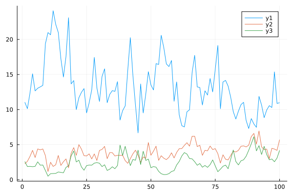
mean(Matrix(res),dims=1)
1×3 Matrix{Float64}:
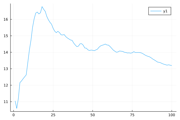
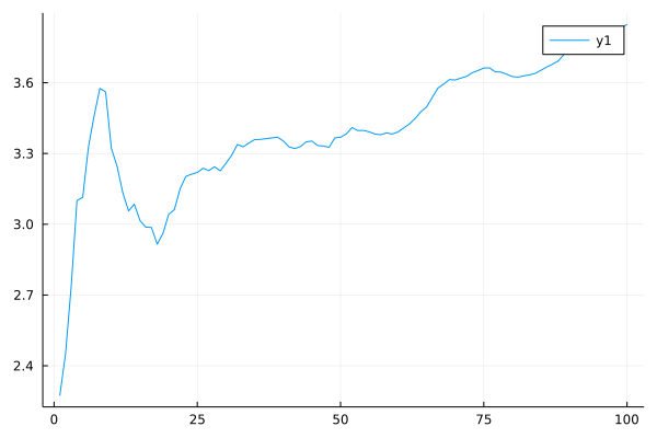
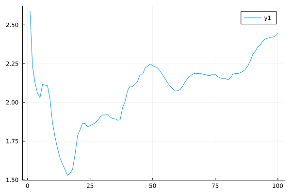
 13.1933  3.8488  2.4452
plot(Matrix(res))
function runMean(x)
    meanx = 0
    [meanx += (v-meanx)/i for (i,v) in enumerate(x)]
end
runMean (generic function with 1 method)
plot(runMean(res[!,1]))
plot(runMean(res[!,2]))
plot(runMean(res[!,3]))
println(mme.randomEffectsVec[1].meanV)
[13.286873876787379 3.9207488622086912; 3.9207488622086912 2.5102330473729233]