
Simple Linear Regression
Contents
15. Simple Linear Regression#
Simple linear regression is used to illustrate Bayesian inference, using the Gibbs sampler. The Gibbs sampler is used to draw samples from the posterior distribution of the intercept, the slope and the residual variance.
15.1. The Model#
Consider the linear model:
where for observation \(i\), \(y_{i}\) is the value of the dependent variable, \(\beta_{0}\) is the intercept, \(x_{i}\) is the value of the independent variable and \(e_{i}\) is a residual. Flat priors are used for the intercept and slope, and the residuals are assumed to be identically and independently distributed normal random variables with mean zero and variance \(\sigma_{e}^{2}.\) A scaled inverted chi-square prior is used for \(\sigma_{e}^{2}.\)
15.2. Simulation of Data#
using Distributions, Printf, Random, Plots
Random.seed!(123)
n = 20 #number of observations
k = 1  #number of covariates
1
X =[ones(n) rand(Binomial(2,0.5), n,k)];
betaTrue = [1,2]
y = X*betaTrue + randn(n);
15.3. Least Squares Estimation#
In matrix notation, the model (1) is
where
Then, the least-squares estimator of \(\mathbf{\beta}\) is
and the variance of this estimator is
15.3.1. Calculations in Julia:#
XPX = X'X
rhs = X'y
XPXi= inv(XPX)
2×2 Matrix{Float64}:
  0.173469  -0.112245
 -0.112245   0.102041
betaHat = XPXi*rhs
2-element Vector{Float64}:
 1.644829033309896
 1.3490913896040329
eHat = y - X*betaHat
resVar = eHat'eHat/(n-2)
1.0999961951362645
15.4. Bayesian Inference#
Consider making inferences about \(\boldsymbol{\beta}\) from \(f(\boldsymbol{\beta}|\mathbf{y},\sigma_{e}^{2}).\) By using the Bayes theorem, this conditional density is written as
which looks like the \(n\)-dimensional normal density of \(\mathbf{y}\) with mean \(\mathbf{X}\boldsymbol{\beta}\) and covariance matrix \(\mathbf{I}\sigma_{e}^{2}.\) But, \(f(\boldsymbol{\beta}|\mathbf{y},\sigma_{e}^{2})\) should be a two-dimensional density. So, the quadratic \(Q=(\mathbf{y}-\mathbf{X}\boldsymbol{\beta})'(\mathbf{y}-\mathbf{X}\boldsymbol{\beta})\) in the exponent of (36) is rearranged as
where \(\hat{\boldsymbol{\beta}}\) is the solution to \((\mathbf{X}'\mathbf{X})\hat{\boldsymbol{\beta}}=\mathbf{X}'\mathbf{y}\), which is the least-squares estimator of \(\boldsymbol{\beta}\). In this expression, only the second term depends on \(\boldsymbol{\beta}\). Thus, \(f(\boldsymbol{\beta}|\mathbf{y},\sigma_{e}^{2})\) can be written as
which can be recognized as proportional to the density for a two-dimensional normal distribution with mean \(\hat{\boldsymbol{\beta}}\) and variance \((\mathbf{X}'\mathbf{X})^{-1}\sigma_{e}^{2}\). Thus, in this simple setting, the posterior mean of \(\boldsymbol{\beta}\) is given by the least-squares estimate, and drawing samples from the posterior are not needed. But, to illustrate the Gibbs sampler, we will apply it to this simple example.
15.4.1. Gibbs Sampler for \(\boldsymbol{\beta}\)#
The simple regression model can be written as
In the Gibbs sampler, \(\beta_{0}\) is sampled from its full-conditional posterior: \(f(\beta_{0}|\mathbf{y},\beta_{1},\sigma_{e}^{2}).\) This conditional distribution is computed for the current values of \(\beta_{1}\) and \(\sigma_{e}^{2}.\) So, we can write the model as
where \(\mathbf{w}_{0}=\mathbf{y}-\mathbf{x}\beta_{1}.\) Then, the least-squares estimator of \(\beta_{0}\) is
and the variance of this estimator is
By applying the strategy used to derive \(f(\boldsymbol{\beta}|\mathbf{y},\sigma_{e}^{2})\) above, the full-conditional posterior for \(\beta_{0}\) can be shown to be a normal distribution with mean \(\hat{\beta_{0}}\) and variance \(\frac{\sigma_{e}^{2}}{\mathbf{1}'\mathbf{1}}\). Similarly, the full-conditional posterior for \(\beta_{1}\) is a normal distribution with mean
and variance \(\frac{\sigma_{e}^{2}}{\mathbf{x}'\mathbf{x}}\), where \(\mathbf{w}_{1}=\mathbf{y}-1\beta_{0}\). In the calculations below, we will use the true value of \(\sigma_{e}^{2}\).
15.4.2. Calculations in Julia:#
niter                 = 100_000       # number of samples
b                     = [0.0, 0.0]    # starting values
samples_b1            = zeros(niter)  # a vector to save MCMC samples for b1
samples_b2            = zeros(niter)  # a vector to save MCMC samples for b2

for iter = 1:niter

    # sampling intercept
    w    = y - X[:,2] * b[2]                  # w0 = y - x2*b2
    x    = X[:,1]                             # x1, a column of 1s
    xpxi = 1/(x'x)                            #
    bHat = (xpxi*x'w)                         # x1'w0/x1'x1
    b[1] = rand(Normal(bHat, sqrt(xpxi*1.0))) # known residual variance = 1

    # sampling slope
    w    = y - X[:,1]*b[1]                    # w1 = y - x1*b1
    x    = X[:,2]                             # x2
    xpxi = 1/(x'x)                            #
    bHat = (xpxi*x'w)                         # x2'w1/x2'x2
    b[2] = rand(Normal(bHat, sqrt(xpxi*1.0))) # known residual variance = 1

    # save MCMC samples from the posterior distribution of b1 and b2
    samples_b1[iter] = b[1]
    samples_b2[iter] = b[2]

    if ((iter%10_000) == 0) #print out posterior mean for b1 and b2
        @printf("Intercept = %6.3f \n", sum(samples_b1)/iter)
        @printf("Slope     = %6.3f \n", sum(samples_b2)/iter)
    end
end
Intercept =  1.645
Slope     =  1.347
Intercept =  1.640
Slope     =  1.352
Intercept =  1.643
Slope     =  1.349
Intercept =  1.647
Slope     =  1.346
Intercept =  1.644
Slope     =  1.349
Intercept =  1.646
Slope     =  1.347
Intercept =  1.647
Slope     =  1.346
Intercept =  1.647
Slope     =  1.347
Intercept =  1.646
Slope     =  1.347
Intercept =  1.646
Slope     =  1.347
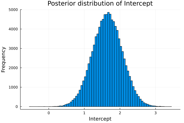
histogram(samples_b1[101:end],
    title  = "Posterior distribution of Intercept",
    ylabel = "Frequency",
    xlabel = "Intercept",
    labels = false
)
15.4.3. Full-conditional Posterior for \(\sigma_{e}^{2}\)#
Recall that we assumed a scaled inverted chi-square prior for \(\sigma_{e}^{2}\). The density function for this is:
where \(S_{e}^{2}\) and \(\nu_{e}\) are the scale and the degrees of freedom parameters for this distribution. Applying Bayes theorem to combine this prior with the “likelihood” (given in (36)), the full-conditional posterior for the residual variance can be written as
Comparing (38) with (37), can see that it is proportional to a scaled inverse chi-squared density with \(\tilde{\nu}_{e}=n+\nu_{e}\) degrees of freedom and \(\tilde{S_{e}^{2}}=\frac{(\mathbf{y}-\mathbf{X}\boldsymbol{\beta})'(\mathbf{y}-\mathbf{X}\boldsymbol{\beta})+\nu_{e}S_{e}^{2}}{\tilde{\nu_{e}}}\) scale parameter. A sample from this density can be obtained as \(\frac{(\mathbf{y}-\mathbf{X}\boldsymbol{\beta})'(\mathbf{y}-\mathbf{X}\boldsymbol{\beta})+\nu_{e}S_{e}^{2}}{\chi_{\tilde{\nu_{e}}}^{2}}\), where \(\chi_{\tilde{\nu_{e}}}^{2}\) is a chi-squared random variable with \(\tilde{\nu_{e}}\) degrees of freedom.
15.4.4. Exercise#
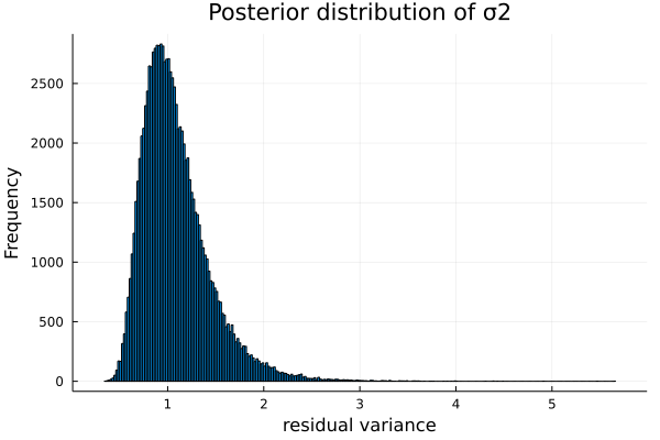
In the Julia script given here, the simulated value of the residual variance was used in the sampling of \(\boldsymbol{\beta}\). Extend this script to also sample \(\sigma_{e}^{2}\) from its full-conditional posterior given above. In Julia, rand(Chisq(\(\nu\))) gives a chi-squared random variable with \(\nu\) degrees of freedom. Solutions can be found below.
niter                 = 100_000       # number of samples
b                     = [0.0, 0.0]    # starting values
samples_b1            = zeros(niter)  # a vector to save MCMC samples for b1
samples_b2            = zeros(niter)  # a vector to save MCMC samples for b2
samples_σ2            = zeros(niter)  # a vector to save MCMC samples for residual variance

###For residual variances
σ2    = 1.0                                  ###
νRes  = 5
S2Res = σ2*(νRes - 2)/νRes
n     = size(X,1)

for iter = 1:niter

    # sampling intercept
    w    = y - X[:,2] * b[2]                  # w0 = y - x2*b2
    x    = X[:,1]                             # x1, a column of 1s
    xpxi = 1/(x'x)                            #
    bHat = (xpxi*x'w)                         # x1'w0/x1'x1
    b[1] = rand(Normal(bHat, sqrt(xpxi*σ2)))  ### unknown residual variance

    # sampling slope
    w    = y - X[:,1]*b[1]                    # w1 = y - x1*b1
    x    = X[:,2]                             # x2
    xpxi = 1/(x'x)                            #
    bHat = (xpxi*x'w)                         # x2'w1/x2'x2
    b[2] = rand(Normal(bHat, sqrt(xpxi*σ2)))  ### unknown residual variance

    # sampling residual variance
    e       = y - X*b                                   ###
    SSE     = e'e                                       ###
    σ2      = (SSE + νRes*S2Res)/rand(Chisq(n+νRes))    ###

    # save MCMC samples from the posterior distribution of b1 and b2
    samples_b1[iter] = b[1]
    samples_b2[iter] = b[2]
    samples_σ2[iter] = σ2

    if ((iter%10_000) == 0) #print out posterior mean for b1 and b2
        @printf("Intercept = %6.3f \n", sum(samples_b1)/iter)
        @printf("Slope     = %6.3f \n", sum(samples_b2)/iter)
        @printf("σ2        = %6.3f \n", sum(samples_σ2)/iter)
    end
end
Intercept =  1.639
Slope     =  1.353
σ2        =  1.082
Intercept =  1.634
Slope     =  1.357
σ2        =  1.085
Intercept =  1.638
Slope     =  1.354
σ2        =  1.087
Intercept =  1.640
Slope     =  1.352
σ2        =  1.086
Intercept =  1.641
Slope     =  1.352
σ2        =  1.085
Intercept =  1.643
Slope     =  1.351
σ2        =  1.086
Intercept =  1.643
Slope     =  1.350
σ2        =  1.085
Intercept =  1.643
Slope     =  1.351
σ2        =  1.086
Intercept =  1.642
Slope     =  1.351
σ2        =  1.086
Intercept =  1.641
Slope     =  1.353
σ2        =  1.086
histogram(samples_σ2[101:end],
    title  = "Posterior distribution of σ2",
    ylabel = "Frequency",
    xlabel = "residual variance",
    labels = false
)
15.5. Model with Normal Prior for Slope#
Here we consider a model with a flat prior for \(\beta_{0}\) and a normal prior for the slope:
where \(\sigma_{\beta}^{2}\) is assumed to be known. Then, the full-conditional posterior for \(\theta'=[\boldsymbol{\beta},\sigma_{e}^{2}]\) is
15.5.1. Full-conditional for \(\beta_{1}\):#
The full-conditional for \(\beta_{1}\) is obtained by dropping all terms and factors that do not involve \(\beta_{1}\):
where
and \(\mathbf{w}=\mathbf{y}-\mathbf{1}\beta_{0}.\) So, the full-conditional posterior for \(\beta_{1}\) is a normal distribution with mean \(\hat{\beta}_{1}\) and variance \(\frac{\sigma_{e}^{2}}{(\mathbf{x}'\mathbf{x}+\sigma_{e}^{2}/\sigma_{\beta}^{2})}.\)
15.5.2. Exercise#
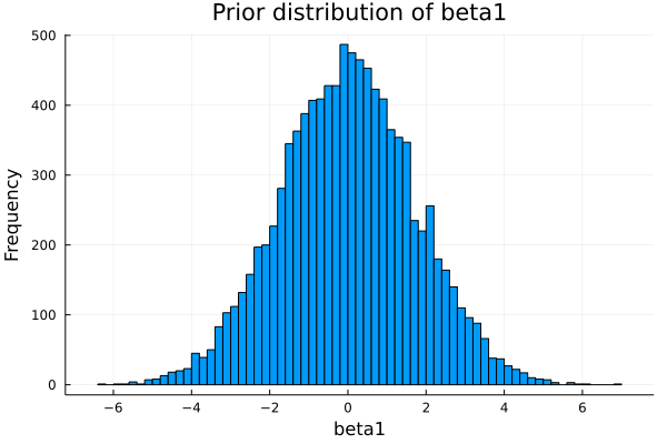
Use Julia to simulate a vector of 10,000 values for \(\beta_{1}\) from a normal distribution with mean zero and variance 3. Use the randn command for this. Plot a histogram of these values.
Using a value of 1 for \(\beta_{0}\) and one of the sampled values of \(\beta_{1}\), generate a vector of observations, \(\mathbf{y},\) that follows a simple linear regression model. Use \(\sigma_{e}^{2}=5\) to simulate \(\mathbf{y}.\)
Use the Gibbs sampler to draw 10,000 samples for \(\beta_{1}\) from its posterior distribution.
Compute the mean and variance of the sampled values.
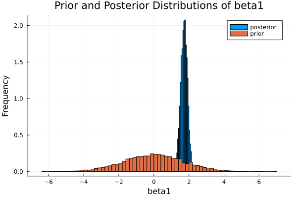
Draw a histogram of the sampled values. Compare with prior.
Use Julia to simulate a vector of 10,000 values for \(\beta_{1}\) from a normal distribution with mean zero and variance 3. Use the randn command for this. Plot a histogram of these values.
15.5.2.1. Prior Distibution of \(\beta_1\)#
prior = randn(10_000)*sqrt(3.0)
histogram(prior,
    title  = "Prior distribution of beta1",
    ylabel = "Frequency",
    xlabel = "beta1",
    labels = false
)
Using a value of 1 for \(\beta_{0}\) and one of the sampled values of \(\beta_{1}\), generate a vector of observations, \(\mathbf{y},\) that follows a simple linear regression model. Use \(\sigma_{e}^{2}=5\) to simulate \(\mathbf{y}.\)
15.5.2.2. Simulation of the data#
Random.seed!(123)
n = 200 # number of observations
k = 1   # number of covariates

x = rand([0,1,2],(n,k))
X = [ones(Int64,n) x]

betaTrue = [1,2]
y        = X*betaTrue+ randn(n)*sqrt(5.0);
Use the Gibbs sampler to draw 10,000 samples for \(\beta_{1}\) from its posterior distribution. 1. Compute the mean and variance of the sampled values. 2. Draw a histogram of the sampled values. Compare with prior.
15.5.3. Posterior Distibution of \(\beta_1\)#
niter                 = 10_000       # number of samples
b                     = [0.0, 0.0]    # starting values
samples_b1            = zeros(niter)  # a vector to save MCMC samples for b1
samples_b2            = zeros(niter)  # a vector to save MCMC samples for b2
samples_σ2            = zeros(niter)  # a vector to save MCMC samples for residual variance

#For residual variances
σ2    = 1.0
νRes  = 5
S2Res = σ2*(νRes - 2)/νRes
n     = size(X,1)

#For random effect β1
vB1   = 3.0                                   ### NEW


for iter = 1:niter
    # sampling intercept
    w    = y - X[:,2] * b[2]                  # w0 = y - x2*b2
    x    = X[:,1]                             # x1, a column of 1s
    xpxi = 1/(x'x)                            #
    bHat = (xpxi*x'w)                         # x1'w0/x1'x1
    b[1] = rand(Normal(bHat, sqrt(xpxi*σ2)))  # unknown residual variance

    # sampling slope
    w    = y - X[:,1]*b[1]                    # w1 = y - x1*b1
    x    = X[:,2]                             # x2
    λ    = σ2/vB1                             ### NEW
    xpxi = 1/(x'x+λ)                          ### NEW
    bHat = (xpxi*x'w)                         # x2'w1/(x2'x2 + Iλ)
    b[2] = rand(Normal(bHat, sqrt(xpxi*σ2)))  # unknown residual variance

    # sampling residual variance
    e       = y - X*b
    SSE     = e'e
    σ2      = (SSE + νRes*S2Res)/rand(Chisq(n+νRes))

    # save MCMC samples from the posterior distribution of b1 and b2
    samples_b1[iter] = b[1]
    samples_b2[iter] = b[2]
    samples_σ2[iter] = σ2

    if ((iter%1_000) == 0) #print out posterior mean for b1 and b2
        @printf("Intercept = %6.3f \n", sum(samples_b1)/iter)
        @printf("Slope     = %6.3f \n", sum(samples_b2)/iter)
        @printf("σ2        = %6.3f \n", sum(samples_σ2)/iter)
    end
end
Intercept =  1.029
Slope     =  1.730
σ2        =  5.220
Intercept =  1.039
Slope     =  1.721
σ2        =  5.217
Intercept =  1.040
Slope     =  1.721
σ2        =  5.214
Intercept =  1.037
Slope     =  1.723
σ2        =  5.224
Intercept =  1.040
Slope     =  1.720
σ2        =  5.224
Intercept =  1.044
Slope     =  1.716
σ2        =  5.224
Intercept =  1.040
Slope     =  1.719
σ2        =  5.223
Intercept =  1.036
Slope     =  1.722
σ2        =  5.226
Intercept =  1.037
Slope     =  1.721
σ2        =  5.227
Intercept =  1.036
Slope     =  1.723
σ2        =  5.225
histogram([samples_b2; prior], group=repeat(["posterior", "prior"],inner=10_000), normalize=true,
    title  = "Prior and Posterior Distributions of beta1",
    ylabel = "Frequency",
    xlabel = "beta1"
)