

Multiple Linear Regression
Contents
16. Multiple Linear Regression#
Consider the multiple regression model
which extends the simple linear regression model in the previous chapter to include multiple covariates \(x_{ij}\). In matrix notation, this model can be written as
where \(\boldsymbol{\beta}'=[\beta_{1},\beta_{2},\ldots,\beta_{k}]\) and the matrix \(\mathbf{X}\) contains the corresponding covariates.
16.1. Model with Normal Prior for Regression Coefficients#
Here we consider a model with iid normal priors for all the slopes:
where \(\sigma_{\beta}^{2}\) is assumed to be known. The residuals are assumed iid normal with null mean and variance \(\sigma_{e}^{2}\), which itself is assigned a scaled inverted chi-square prior. Then, the joint posterior for \(\boldsymbol{\theta}\) is
The posterior distribution for \(\boldsymbol{\beta}\) can be written as
for
where \(\mathbf{D}\) is a diagonal matrix with ones on the diagonals. Thus, the full-conditional posterior for \(\boldsymbol{\beta}\) is a normal distribution with mean given by (2) and variance \((\mathbf{X}'\mathbf{X}+\mathbf{D}\frac{\sigma_{e}^{2}}{\sigma_{\beta}^{2}})^{-1}\sigma_{e}^{2}.\)
16.1.1. Full-conditionals:#
The full conditionals for \(\sigma_{e}^{2}\) are identical to those in simple linear regression.
16.1.2. Full-conditional for \(\beta_{j}\)#
The full-conditional for \(\beta_{j}\) is obtained by dropping from the joint posterior all terms and factors that do not involve \(\beta_{j}\):
where
and \(\mathbf{w}_{j}=\mathbf{y}-\sum_{l\neq j}\mathbf{x}_{l}\beta_{l}.\) So, the full-conditional posterior for \(\beta_{j}\) is a normal distribution with mean \(\hat{\beta}_{j}\) and variance \(\frac{\sigma_{e}^{2}}{(\mathbf{x}_{j}'\mathbf{x}_{j}+\sigma_{e}^{2}/\sigma_{\beta}^{2})}.\)
16.1.3. Exercise#
Generate data from model (1) with \(k=10\) covariates.
Setup and solve the mixed model equations given by (2).
Sample the elements of \(\boldsymbol{\beta}\) using Gibbs.
Compute the posterior mean of \(\boldsymbol{\beta}\) from the samples and compare with mixed model solutions.
Compute the posterior covariance matrix from the sampled values. Compare results with inverse of the mixed-model coefficient matrix.
using Distributions, Printf, LinearAlgebra, ProgressMeter, Random
1 . Generate data from model (1) with 𝑘=10 covariates.
Random.seed!(31415)
n        = 2000                       #number of observations
k        = 10                         #number of covariates
M        = rand(Binomial(2,0.5),n,k)
X        = M .- mean(M,dims=1);
betaTrue = randn(k)
y        = X*betaTrue+ randn(n)*1.0;  #residual variance = 1.0
Setup and solve the mixed model equations given by (2).
XPX = X'X
rhs = X'y
Vb  = var(betaTrue)
Ve  = 1
λ   = Ve/Vb
mme = XPX
mme += I*λ;
betaHat=inv(mme)*rhs
10-element Vector{Float64}:
 -0.5011910347406648
 -0.5782245478425588
  1.0891494613977095
  0.8884697817770406
 -0.13606917962763193
  0.4329405585028446
 -1.609666927677
 -0.8358922263166609
  0.142828510272148
  1.3078902050561971
Sample the elements of 𝜷 using Gibbs.
function GibbsSample1(y,X,b,niter,λ)
    n,k     = size(X)
    samples = zeros(niter,k)
     @showprogress "drawing MCMC samples..." for iter = 1:niter
        for i=1:k
            btemp    = copy(b)
            btemp[i] = 0
            w        = y - X*btemp                        # wj
            x        = X[:,i]                             # xj
            xpxi     = 1/((x'x) + λ)                      # 1/(xj'xj+(σ_e)^2/(σ_b)^2)
            bHat     = (xpxi*x'w)                         # 1/(xj'xj+(σ_e)^2/(σ_b)^2) * xj'wj
            b[i]     = rand(Normal(bHat, sqrt(xpxi*1.0))) # known residual variance = 1.0
        end
        samples[iter,:] = b
    end
    return samples
end
GibbsSample1 (generic function with 1 method)
Compute the posterior mean of 𝜷 from the samples and compare with mixed model solutions.
niter = 1000                    # number of MCMC samples
b     = zeros(k)
@time samples = GibbsSample1(y,X,b,niter,λ);
drawing MCMC samples... 100%|████████████████████████████| Time: 0:00:00
0.742187 seconds (666.52 k allocations: 496.511 MiB, 5.99% gc time, 15.58% compilation time)
meanb=vec(mean(samples,dims=1))
[meanb betaHat]
10×2 Matrix{Float64}:
 -0.501586  -0.501191
 -0.578543  -0.578225
  1.09022    1.08915
  0.888518   0.88847
 -0.134843  -0.136069
  0.43311    0.432941
 -1.6106    -1.60967
 -0.836354  -0.835892
  0.141131   0.142829
  1.30602    1.30789
Compute the posterior covariance matrix from the sampled values. Compare results with inverse of the mixed-model coefficient matrix.
covMat_bayes=cov(samples)
10×10 Matrix{Float64}:
  0.000939535   1.4766e-5    -2.28614e-5   …  -4.89595e-5  -4.78057e-5
  1.4766e-5     0.000945363   2.18577e-6       3.25844e-5  -2.21268e-5
 -2.28614e-5    2.18577e-6    0.000994687      2.16452e-5   5.05519e-5
 -2.69692e-5   -4.86041e-5   -2.20135e-5      -6.82278e-5   6.02622e-5
  1.697e-5      2.73304e-5    5.13688e-6       7.03594e-6  -1.09161e-6
  3.281e-5      4.73932e-5    2.84289e-5   …  -8.33934e-6  -7.7537e-5
  6.0638e-6     6.60487e-5   -2.18976e-5       3.67536e-5  -5.57869e-5
  2.60998e-5   -4.59133e-5    1.71669e-5      -3.30883e-5  -2.00971e-5
 -4.89595e-5    3.25844e-5    2.16452e-5       0.00101303   2.26448e-5
 -4.78057e-5   -2.21268e-5    5.05519e-5       2.26448e-5   0.00106718
covMat_freq=inv(mme)
10×10 Matrix{Float64}:
  0.00101185  -1.19064e-6  -1.63284e-5   …  -6.96065e-6  -2.79695e-5
 -1.19064e-6   0.00100676  -6.62762e-6       2.61475e-6  -2.47689e-5
 -1.63284e-5  -6.62762e-6   0.000998215     -3.15949e-5  -3.50533e-6
 -4.25714e-6   6.82698e-6  -1.46198e-5      -4.00477e-5   1.50206e-5
 -1.12512e-5   2.51804e-5   2.28552e-5      -2.03058e-6   1.21646e-5
  3.80437e-5   3.90624e-5   1.47221e-5   …  -2.09811e-5  -5.36175e-5
 -1.63895e-5   7.02744e-6  -1.38133e-6       7.59088e-5  -2.78627e-5
  2.1496e-6   -5.85011e-5  -9.53933e-7       6.95683e-6  -3.16674e-5
 -6.96065e-6   2.61475e-6  -3.15949e-5       0.00102316   1.35484e-5
 -2.79695e-5  -2.47689e-5  -3.50533e-6       1.35484e-5   0.00100619
round.(covMat_bayes-covMat_freq,digits=2)
10×10 Matrix{Float64}:
 -0.0   0.0  -0.0  -0.0   0.0  -0.0   0.0   0.0  -0.0  -0.0
  0.0  -0.0   0.0  -0.0   0.0   0.0   0.0   0.0   0.0   0.0
 -0.0   0.0  -0.0  -0.0  -0.0   0.0  -0.0   0.0   0.0   0.0
 -0.0  -0.0  -0.0   0.0  -0.0  -0.0   0.0   0.0  -0.0   0.0
  0.0   0.0  -0.0  -0.0   0.0  -0.0   0.0   0.0   0.0  -0.0
 -0.0   0.0   0.0  -0.0  -0.0   0.0   0.0   0.0   0.0  -0.0
  0.0   0.0  -0.0   0.0   0.0   0.0   0.0  -0.0  -0.0  -0.0
  0.0   0.0   0.0   0.0   0.0   0.0  -0.0  -0.0  -0.0   0.0
 -0.0   0.0   0.0  -0.0   0.0   0.0  -0.0  -0.0  -0.0   0.0
 -0.0   0.0   0.0   0.0  -0.0  -0.0  -0.0   0.0   0.0   0.0
16.2. Model with unknown \(\sigma_{\beta}^{2}\) (RR-BLUP)#
In the previous section, we assumed that \(\sigma_{\beta}^{2}\) in the prior of the slopes was known. Here, we will consider this variance to be unknown with a scaled inverted chi-square prior with scale parameter \(S_{\beta}^{2}\) and degrees of freedom \(\nu_{\beta}.\) The joint posterior for this model is
Then, the full-conditional posterior for \(\sigma_{\beta}^{2}\) is
which can be recognized as a scaled inverted chi-square distribution with \(\tilde{\nu}_{\beta}=k+\nu_{\beta}\) degrees of freedom and scale parameter \(\tilde{S}_{\beta}^{2}=(\sum_{j=1}^{k}\beta_{j}^{2}+\nu_{\beta}S_{\beta}^{2})/\tilde{\nu}_{\beta}.\) A sample from this posterior can be obtained as \(\frac{\sum_{j=1}^{k}\beta_{j}^{2}+\nu_{\beta}S_{\beta}^{2}}{\chi_{\tilde{\nu}_{\beta}}^{2}}\).
16.2.1. Exercise#
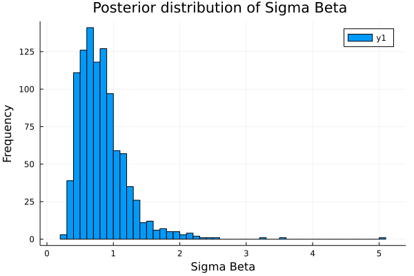
Extend the sampler used in the previous section to treat \(\sigma_{\beta}^{2}\) as an unknown. Plot the posterior distribution for \(\sigma_{\beta}^{2}\).
function GibbsSample2(y,X,b,niter,νB,Sb)
    n,k          = size(X)
    samplesb     = zeros(niter,k)
    samples_varb = zeros(niter)
    λ            = 1.0                                        ###
    @showprogress "drawing MCMC samples..." for iter = 1:niter
        for i=1:k
            btemp    = copy(b)
            btemp[i] = 0
            w        = y - X*btemp                        # wj
            x        = X[:,i]                             # xj
            xpxi     = 1/((x'x) + λ)                      # 1/(xj'xj+(σ_e)^2/(σ_b)^2)
            bHat     = (xpxi*x'w)                         # 1/(xj'xj+(σ_e)^2/(σ_b)^2) * xj'wj
            b[i]     = rand(Normal(bHat, sqrt(xpxi*1.0))) # known residual variance = 1.0
        end

        # sampling (σ_b)^2
        varb = (sum(b.^2) + νB*Sb) /rand(Chisq(νB+k))     ###
        λ    = 1.0/varb                                   ###


        samplesb[iter,:]   = b
        samples_varb[iter] = varb
    end
    return samples_varb
end
GibbsSample2 (generic function with 1 method)
niter = 1000                     # number of samples
b     = zeros(k)
νB    = 4
varb  = 1
vare  = 1
Sb    = varb*(νB - 2)/νB
@time samples_varb = GibbsSample2(y,X,b,niter,νB,Sb);
drawing MCMC samples... 100%|████████████████████████████| Time: 0:00:00
0.788078 seconds (119.23 k allocations: 467.112 MiB, 6.86% gc time, 4.41% compilation time)
using Plots
histogram(samples_varb,
title  = "Posterior distribution of Sigma Beta ",
ylabel = "Frequency",
xlabel = "Sigma Beta"
)
16.3. Model with unknown covariate-specific variances (BayesA)#
Here we consider a model where the prior for the slope corresponding to covariate \(j\) is normal with mean 0 and variance \(\sigma_{j}^{2}\), where \(\sigma_{j}^{2}\) has scaled inverted chi-square prior with scale parameter \(S_{\beta}^{2}\) and degrees of freedom \(\nu_{\beta}.\) The joint posterior for this model is
It can be shown that:
The full-conditional posterior for \(\beta_{j}\) is normal with mean
\[ \hat{\beta}_{j}=\frac{\mathbf{x}_{j}'\mathbf{w}_{j}}{(\mathbf{x}_{j}'\mathbf{x}_{j}+\sigma_{e}^{2}/\sigma_{j}^{2})}, \]and variance \(\frac{\sigma_{e}^{2}}{(\mathbf{x}_{j}'\mathbf{x}_{j}+\sigma_{e}^{2}/\sigma_{j}^{2})}\).
The full-conditional posterior for \(\sigma_{j}^{2}\) is a scaled inverted chi-square distribution with \(\tilde{\nu}_{\beta}=1+\nu_{\beta}\) degrees of freedom and scale parameter \(\tilde{S}_{\beta}^{2}=(\beta_{j}^{2}+\nu_{\beta}S_{\beta}^{2})/\tilde{\nu}_{\beta}.\) A sample from this posterior can be obtained as \(\frac{\beta_{j}^{2}+\nu_{\beta}S_{\beta}^{2}}{\chi_{\tilde{\nu}_{\beta}}^{-2}}\).
Marginally, the prior for \(\beta_{j}\) is a scaled \(t\) distribution with \(\nu_{\beta}\) degrees of freedom, mean 0 and scale parameter \(S_{\beta}^{2}.\)
16.4. Model with unknown \(S^2_{\beta}\)#
The conjugate prior for \(S^2_{\beta}\) is the gamma distribution, and following Habier et al. (2011), we will use a Gamma(1,1) prior. The pdf of the gamma is:
In the joint posterior, \(S^2_{\beta}\) only appears in the prior for \(\sigma^2_j\), which is a scaled inverted chi-square distribution with pdf: $\( \prod_{j=1}^{k} \frac{(S^2_{\beta}\nu_{\beta}/2)^{\nu_{\beta}/2}}{\Gamma(\nu_{\beta}/2)}\left(\sigma_{j}^{2}\right)^{-(2+\nu_{\beta})/2}\exp\left\{ -\frac{\nu_{\beta}S_{\beta}^{2}}{2\sigma_{j}^{2}}\right\} \)$
Combining these two densities, the full conditional posterior for \(S^2_{\beta}\) can be written as:
Comparing this with the gamma density given above, shows that the full conditional posterior for \(S^2_{\beta}\) is a gamma distribution with \(\alpha = k\nu_{\beta}/2 + 1\) and \(\beta = 1 + \sum_j^k (\frac{\nu_{\beta}}{2\sigma^2_j})\).
16.5. Model with Mixture Prior for Regression Coefficients (BayesC)#
As before, a flat prior is used for the intercept, \(\mu\). The prior for slope \(j\) is a mixture:
where \(\sigma_{\beta}^{2}\) has a scaled inverted chi-square prior with scale parameter \(S_{\beta}^{2}\) and degrees of freedom \(\nu_{\beta}.\) In order to use the Gibbs sampler, it is convenient to write \(\beta_{j}\) as
where \(\delta_{j}\) is a Bernoulli variable with probability \(1-\pi\) of being 1:
and \(\gamma_{j}\) is normally distributed with mean zero and variance \(\sigma_{\beta}^{2}.\) Then, the model for the phenotypic values can be written as $\(y_{i}=\mu+\sum_{j=1}X_{ij}\gamma_{j}\delta_{j}+e_{i}.\)$
16.5.1. Full-conditionals:#
The joint posterior for all the parameters is proportional to
where \(\boldsymbol{\theta}\) denotes all the unknowns.
16.5.2. Full-conditional for \(\mu\)#
The full-conditional for \(\mu\) is a normal distribution with mean \(\hat{\mu}\) and variance \(\frac{\sigma_{e}^{2}}{n}\), where \(\hat{\mu}\) is the least-squares estimate of \(\mu\) in the model
and \(\frac{\sigma_{e}^{2}}{n}\) is the variance of this estimator (\(n\) is the number of observations).
16.5.3. Full-conditional for \(\gamma_{j}\)#
where
So, the full-conditional for \(\gamma_{j}\) is a normal distribution with mean
and variance \(\frac{\sigma_{e}^{2}}{(\mathbf{x}'_{j}\mathbf{x}_{j}\delta_{j}+\sigma_{e}^{2}/\sigma_{\beta}^{2})}\).
16.5.4. Full-conditional for \(\delta_{j}\)#
where $\(h(\delta_{j})=\pi^{(1-\delta_{j})}(1-\pi)^{\delta_{j}}\exp\left\{ -\frac{ (\mathbf{w}_{j}-\mathbf{X}_{j}\gamma_{j}\delta_{j})' (\mathbf{w}_{j}-\mathbf{X}_{j}\gamma_{j}\delta_{j}) }{2\sigma_{e}^{2}}\right\} .\)$
16.5.5. Full-conditional for \(\sigma_{\beta}^{2}\)#
and this is proportional to a scaled inverted chi-square distribution with \(\tilde{\nu}_{\beta}=\nu_{\beta}+k\) and scale parameter \(\tilde{S}_{\beta}^{2}=(\sum_{j=1}^{k}\gamma_{j}^{2}+\nu_{\beta}S_{\beta}^{2})/\tilde{\nu}_{\beta}\).
16.5.6. Full-conditional for \(\pi\)#
which is proportional to a Beta distribution with parameters \(a=k-\sum_{j=1}^{k}\delta_{j}+1\) and \(b=\sum\delta_{j}+1.\)
16.5.7. Full-conditional for \(\sigma_{e}^{2}\)#
which is proportional to a scaled inverted chi-square density with \(\tilde{\nu}_{e}=n+\nu_{e}\) degrees of freedom and \(\tilde{S_{e}^{2}}=\frac{(\mathbf{y}-\mathbf{1}\mu-\sum\mathbf{X}_{j}\gamma_{j}\delta_{j})'(\mathbf{y}-\mathbf{1}\mu-\sum\mathbf{X}_{j}\gamma_{j}\delta_{j})+\nu_{e}S_{e}^{2}}{\tilde{\nu_{e}}}\) scale parameter.