2. Introduction to Bayesian Inference#

2.1. Bayes’ Theorem#

2.1.1. Motivation#

In whole-genome analyses, the number $k$ of marker covariates typically exceeds the number of $n$ of observations. In this situation, least squares methods cannot be used to simultaneously estimate the effects of all the $k$ marker covariates. One of the most widely used methods to overcome this problem is Bayesian inference, where prior information about marker effects is combined with the data to make inferences about the marker effects. In Bayesian inference, inferences are based on conditional probabilities, and the Bayes theorem is a statement on conditional probability.

2.1.2. Conditional Probability of $X$ Given $Y$#

Suppose $X$ and $Y$are two random variables with joint probability distribution $\Pr(X,Y)$. Then, the conditional probability of $X$ given $Y$ is given by Bayes theorem as

\[ \Pr(X|Y) = \frac{\Pr(X,Y)}{\Pr(Y)} \tag{1} \]

where $\Pr(Y)$ is the probability distribution of $Y$. Similarly, the the conditional probability of $Y$ given $X$ is

\[ \Pr(Y|X)=\frac{\Pr(X,Y)}{\Pr(X)}, \]

which upon rearranging gives

\[\Pr(X,Y)=\Pr(Y|X)\Pr(X). \tag{2}\]

Then, substituting (2) in (1) gives

\[\begin{split}\begin{eqnarray} \Pr(X|Y) &= &\frac{\Pr(X,Y)}{\Pr(Y)}\\ &= &\frac{\Pr(Y|X)\Pr(X)}{\Pr(Y)}, \end{eqnarray}\end{split}\]

which is the form of the formula that is used for inference of $X$ given $Y.$

2.1.3. Bayes’ Theorem by Example#

Here we consider a simple example to justify the formula (1). The following table gives the joint distribution of smoking and lung cancer in a hypothetical population of 1,000,000 individuals.

\[\begin{split} \begin{array}{c|lcr} n & \text{Yes (Smoke)} & \text{No (Smoke)} & \\ \hline \text{Yes (Cancer)} & 42,500 & 7,500 & 50,000 \\ \text{No (Cancer)} & 207,500 & 742,500 & 950,000 \\ & 250,000 & 750,000 & 1,000,000 \end{array} \end{split}\]

Given these numbers, consider how you would compute the relative frequency of lung cancer among smokers.

There are a total of 250,000 smokers in this population, and among these 250,000 individuals, 42,500 have lung cancer. So, relative frequency of lung cancer among smokers is $\frac{42,500}{250,000}$.

As we reason below, this relative frequency is also the conditional probability of lung cancer given the individual is a smoker.

The frequentist definition of probability of an event is the limiting value of its relative frequency in a “large” number of trials.
Suppose we sample with replacement individuals from the 250,000 smokers and compute the relative frequency of the incidence of lung cancer.
It can be shown that as the sample size goes to infinity, this relative frequency will approach $\frac{42,500}{250,000}=0.17$.
This ratio can also be written as

\[\frac{42,500/1,000,000}{250,000/1,000,000}=0.17.\]
The ratio in the numerator is the joint probability of smoking and lung cancer, and the ratio in the denominator is the marginal probability of smoking.

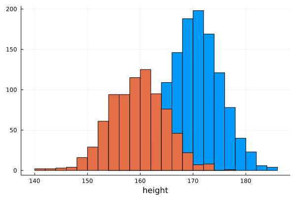
2.1.3.1. Simulated Data for Human Height#

using Plots,Statistics,DataFrames, Random

Random.seed!(123)
mean_male   = 170
sd_male     = 5
mean_female = 159
sd_female   = 5
nind_male   = 1200
nind_female = 800
males       = mean_male .+ randn(nind_male)*sd_male
females     = mean_female .+ randn(nind_female)*sd_female
data=[convert.(Int,round.(males))  fill("male",nind_male)
      convert.(Int,round.(females)) fill("female",nind_female)];
data = DataFrame(height=data[:,1],gender=data[:,2])
first(data,5)

5 rows × 2 columns

	height	gender
	Any	Any
1	174	male
2	164	male
3	164	male
4	168	male
5	171	male

plot(data[data[!,:gender].=="male",:height],seriestype=:histogram,xlabel=:height,legend=:none) 
plot!(data[data[!,:gender].=="female",:height],seriestype=:histogram) 

../_images/6.0.IntroductionBayesianInference_5_0.svg

2.1.3.2. Questions#

Consider the population simulated above. For a randomly sampled person of height equal to 150cm, what is the probability for the person being a female?
1. What is the joint probability for a randomly sampled person to be of height 150cm and a female?
2. What is the marginal probability for a randomly sampled person to be of height 150cm?
3. What is the conditional probability for a person being a female given that the person’s height is 150cm?
Repeat question 1 for a randomly sampled person of height:
1. equal to 170cm
2. equal to 180cm
3. larger than 170cm

2.1.3.3. Julia commands useful for excercise#

height=170

num_joint=count((data[!,:height].> height) .& (data[!,:gender] .== "female"))

den_joint=size(data,1)

p_joint = num_joint/den_joint

0.007

num_mar=count((data[!,:height].== height))
den_mar=size(data,1)
p_mar=num_mar/den_mar

0.056

p_cond = p_joint/p_mar

0.125

2.2. Bayesian Inference#

2.2.1. Meaning of Probability in Bayesian Inference#

In the frequentist approach, probability is a limiting frequency. Thus, probabilities are always associated with random events. In Bayesian inference, on the other hand, probability is used to quantify your belief that an unobservable variable has a particular value. For example a Bayesian can ask questions such as:

What is the probability that heritability for milk yield is larger than 0.5?
What is the probability that variability in milk yield is due to more than 100 loci?

These Bayesian probabilities are not necessarily associated with a random experiment that assigns values to the variables in question.

2.2.2. Essential Elements of Bayesian Inference#

Bayesian inference starts by specifying what you believe about the parameters or unknowns through prior probabilities. In whole-genome analyses, we will use a prior probability density to quantify our belief that the effect of most marker covariates is zero or close to zero and only a few covariates have effects that deviate from zero.
These parameters are related to the data through the model or “likelihood”, which are conditional probabilities for the data given the parameters. In whole-genome analyses, this is usually a multiple regression model with normally distributed residuals.
The prior and the likelihood are combined using Bayes theorem to obtain posterior probabilities, which are conditional probabilities for the parameters given the data.
Inferences about the parameters are based on the posterior.

2.2.3. Use of Bayes Theorem#

Let $f(\boldsymbol{\theta)}$ denote the prior probability density for $\boldsymbol{\theta}$.
Let $f(\boldsymbol{y}|{\boldsymbol{\theta}})$ denote the likelihood
Then, the posterior probability of $\boldsymbol{\theta}$ is:

\[\begin{split}\begin{eqnarray} f({\boldsymbol \theta}|{\boldsymbol y}) & =\frac{f({\boldsymbol y}|{\boldsymbol \theta})f({\boldsymbol \theta})}{f({\boldsymbol y})}\\ & \propto f({\boldsymbol y}|{\boldsymbol \theta})f({\boldsymbol \theta}) \end{eqnarray}\end{split}\]

2.3. Markov Chain Monte-Carlo Methods#

Often no closed form for $f({\boldsymbol \theta}|{\boldsymbol y})$
Further, even if computing $f({\boldsymbol \theta}|{\boldsymbol y})$ is feasible, obtaining $f(\theta_{i}|{\boldsymbol y})$ would require integrating over many dimensions
Thus, in many situations, inferences are made using the empirical posterior constructed by drawing samples from $f({\boldsymbol \theta}|{\boldsymbol y})$
Gibbs sampler is widely used for drawing samples from posteriors

2.3.1. Gibbs Sampler#

Want to draw samples from $f(x_{1},x_{2},\ldots,x_{n})$
Even though it may be possible to compute $f(x_{1},x_{2},\ldots,x_{n})$, it is difficult to draw samples directly from $f(x_{1},x_{2},\ldots,x_{n})$
Gibbs:
- Get valid a starting point $\mathbf{x}^{0}$
- Draw sample $\mathbf{x}^{t}$ as: $$\begin{matrix}x_{1}^{t} & \text{from} & f(x_{1}|x_{2}^{t-1},x_{3}^{t-1},\ldots,x_{n}^{t-1})\\ x_{2}^{t} & \text{from} & f(x_{2}|x_{1}^{t},x_{3}^{t-1},\ldots,x_{n}^{t-1})\\ x_{3}^{t} & \text{from} & f(x_{3}|x_{1}^{t},x_{2}^{t},\ldots,x_{n}^{t-1})\\ \vdots & & \vdots\\ x_{n}^{t} & \text{from} & f(x_{n}|x_{1}^{t},x_{2}^{t},\ldots,x_{n-1}^{t}) \end{matrix}$$
The sequence $\mathbf{x}^{1},\mathbf{x}^{2},\ldots,\mathbf{x}^{t}$ is a Markov chain with stationary distribution $f(x_{1},x_{2},\ldots,x_{n})$

2.3.2. Making Inferences from Markov Chain#

Can show that samples obtained from a Markov chain can be used to draw inferences from $f(x_{1},x_{2},\ldots,x_{n})$ provided the chain is:

Irreducible: can move from any state $i$ to any other state $j$
Positive recurrent: return time to any state has finite expectation
Markov Chains, J. R. Norris (1997)

2.3.3. Exercise#

Let $f(x)$ be a bivariate normal density with means

\[\begin{split} \mathbf{\mu} = \begin{bmatrix} 1\\ 2\\ \end{bmatrix} \end{split}\]

and covariance matrix

\[\begin{split} \mathbf{V} = \begin{bmatrix} 1.0 & 0.5\\ 0.5 & 2.0\\ \end{bmatrix} \end{split}\]

Suppose we don’t know how to draw samples from $f(\mathbf{x})$, but know how to sample from $f(x_i|x_j)$, which is univariate normal with mean:

\[ \mu_{i.j}=\mu_i+\frac{V_{ij}}{V_{jj}}(x_j-\mu_j) \]

and variance

\[ V_{i.j}=V_{ii}-\frac{V^2_{ij}}{V_{jj}} \]

Gibbs
- Start with $\mathbf{x}^{0}=\begin{bmatrix}0\\0\\\end{bmatrix}$
- Draw samples $\mathbf{x}^{t}$ as:
  - $x_1^t$ from $f(x_1|x_2^{t-1})$
  - $x_2^t$ from $f(x_2|x_1^{t})$
- Use the sequence of $\mathbf{x}^1,\mathbf{x}^2,\cdots,\mathbf{x}^n$ to compute any property of $\mathbf{x}$, for example
  - $Pr(x_1 > 1 \text{ and } x_2 > 2)$

Suppose we don’t know how to draw samples from $f(\mathbf{x})$, but know how to sample from $f(x_1|x_2)$, which is univariate normal with mean:

\[ \mu_{1.2}=\mu_1+\frac{V_{12}}{V_{22}}(x_2-\mu_2) \]